Principal plane
Definitions
definition of the equivalent refracting locus, the principal plane and the principal point definition of back / front
computing a principal plane when:
- there is no defined light source nor fixed image plane
- focal length is not known (because the system doesn't have any paraxial information)
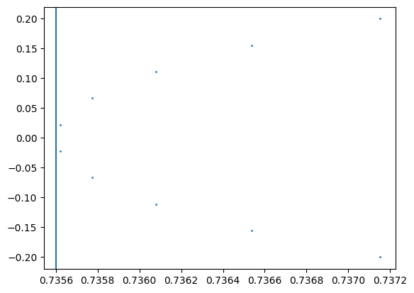
Computing the intersection of input and output rays to a sequential system is easy. The difficult part is that the principal point is defined as the limit of that intersection as the incident ray height goes to zero. The intersection itself is undefined at zero.
To do this, we fit a parabola
Then, the principal point is the vertex of the best fit parabola:
Splitting the chain
Problem:
how to compute the front principal point? Need a way to "invert" an optical sequence.
- Invert the optical sequence
- Keep the kinematic sequence the same
Insight: the kinematic sequence doesn't depend on the optical one but the optical sequence depends on the kinematic one, because surface positions / tf are on the kinematic chain
Idea: evaluate the kinematic chain first, this creates a realization of the chain, so positions are known Can now evaluate the optical chain, forward or backwards
splitting the tf and optics chain
kinematic data = just tf chain kinematic elements = operate on kinematic data
optical data = just ray info optical elements = operate on optical data, also gets tf info somehow
collision surface?
- evaluate kinematic model with forward_tree or similar
- evaluate optics model, giving realized tf
how to associate realized tf to optical elements?
using forward tree, I can associate the outputs of a sequential of kinematic element to module in the sequence but need to associate to modules of another sequence, the optical sequence
indexing probably the best: straightforward, reversible
optical data contains static info on the realized tf chain: a list of length N what if we have a non linear tf tree, like a fork?
general case
first pass: evaluate kinematic model get a realized tf tree, bound to variables second pass: evaluate the optical model, passing ray data and needed tf data
sequential special case
first pass: evaluate kinematic model, results in a list of list of tf, length N the realized tf tree is stored in a list (list of list to handle absolute transform resets) second pass: evaluate the optical model, passing ray data and tf list elements
Kinematic Elements: def forward(chain: KinematicChain) -> KinematicChain
Optical Element: def forward(rays: RayBundle, tf: TransformBase) -> RayBundle
how to do collision surface? one module should be able to act as both kinematic and optical forward_kinematic() forward_optical()
collision surface actually output two tf:
- the one that applies to the held surface
- the one that applis to the next element in the kinematic chain
or fully split collision surface:
SurfaceAnchor: KinematicElement def forward(chain: KinematicChain) -> tuple[KinematicChain, KinematicChain]
RefractiveOpticalSurface: OpticalElement def forward(rays: RaysBundle, tf: TransformBase) -> RayBundle
class RefractiveSurface: def init: self.anchor_surface self.collision_surface self.material
def sequential(inputs):
    # kinematic step:
        # compute tf using anchor surface
    # optical step:
        # compute collisions using collision surface at tf
        # compute refraction
    return outputs

    # split sequential() into kinematic step and optical step?
    # outputs of the kinematic step are given as input to the optical step

    # this enables reverse optical mode:
    #    call sequential kinematic steps in normal order
    #    store outputs indexed by the module
    #    call optical steps in reverse order, getting the correct tf inputs for each optical step
in general: elements forward functions do what makes sense sequential element figures it out to make sequential mode convinient / or elements have a sequential() version of their forward function
how to use mixed style elements into a sequential?
sequential can have logic: if (kinematic element) give it tf if (optical) give it rays if (mixed) give it both
Sequential elements can contribute to either or both chains
complete model is always a kinematic model and an optical model
inverting = invert the optical model, keep the kinematic model
"Main loop": Forward kinematic chain -> Obtain a tf for each element of the optical chain Forward optical chain
A mixed element is an alias constructor for putting an element on both chains
sequential syntax returns a SequentialModel that's made of a kinematic and optical model
tlm.RefractiveSurface(...) # returns a kinematic and an optical model
class Sequential: kinematic model: Sequential of KinematicElement optical model: Sequential of OpticalElement # how to give the right tf to each optical element? # both have same length, use index # or optical element is stored next to an index of corresponding kinematic element
how to do recursive sequential?
import torch
import torchlensmaker as tlm

doublet = tlm.Sequential(
    tlm.RefractiveSurface(tlm.Sphere(4.0, C=0.135327), material=tlm.NonDispersiveMaterial(1.517)),
    tlm.Gap(1.05),
    tlm.RefractiveSurface(tlm.Sphere(4.0, C=-0.19311), material=tlm.NonDispersiveMaterial(1.649)),
    tlm.Gap(0.4),
    tlm.RefractiveSurface(tlm.Sphere(4.0, C=-0.06164), material="air"),
)

optics = tlm.Sequential(
    tlm.PointSourceAtInfinity(3.0),
    tlm.Gap(2),
    doublet,
    #tlm.Gap(2), # use an element for end=?
)

tlm.show(optics, dim=2, controls={"show_optical_axis": True}, end=2)


def back_principal_point(optics):
    """
    Back principal point of a sequential system

    Returns a coordinate along the optical axis (the X axis in TLM convention),
    expressed in the sequential system kinematic frame
    """

    ...


raw_inputs = tlm.default_input(dim=2, dtype=torch.float64, sampling={"base": 10})

# diameter of the sequential system
diameter = 4.0

inputs = tlm.PointSourceAtInfinity(diameter / 10)(raw_inputs)
print(inputs.P.shape)

outputs = doublet(inputs)
print(outputs.P.shape)

print(outputs)
torch.Size([10, 2])
torch.Size([10, 2])
OpticalData(dim=2, dtype=torch.float64, sampling={'base': DenseSampler(size=10)}, dfk=tensor([[1.0000, 0.0000, 1.4500],
[0.0000, 1.0000, 0.0000],
[0.0000, 0.0000, 1.0000]], dtype=torch.float64), ifk=tensor([[ 1.0000, 0.0000, -1.4500],
[ 0.0000, 1.0000, 0.0000],
[ 0.0000, 0.0000, 1.0000]], dtype=torch.float64), P=tensor([[ 1.4489, -0.1881],
[ 1.4493, -0.1463],
[ 1.4497, -0.1045],
[ 1.4499, -0.0627],
[ 1.4500, -0.0209],
[ 1.4500, 0.0209],
[ 1.4499, 0.0627],
[ 1.4497, 0.1045],
[ 1.4493, 0.1463],
[ 1.4489, 0.1881]], dtype=torch.float64), V=tensor([[ 0.9999, 0.0167],
[ 0.9999, 0.0130],
[ 1.0000, 0.0093],
[ 1.0000, 0.0056],
[ 1.0000, 0.0019],
[ 1.0000, -0.0019],
[ 1.0000, -0.0056],
[ 1.0000, -0.0093],
[ 0.9999, -0.0130],
[ 0.9999, -0.0167]], dtype=torch.float64), rays_base=tensor([-0.2000, -0.1556, -0.1111, -0.0667, -0.0222, 0.0222, 0.0667, 0.1111,
0.1556, 0.2000], dtype=torch.float64), rays_object=None, rays_image=None, rays_wavelength=None, var_base=tensor([-0.2000, -0.1556, -0.1111, -0.0667, -0.0222, 0.0222, 0.0667, 0.1111,
0.1556, 0.2000], dtype=torch.float64), var_object=None, var_wavelength=None, material=<torchlensmaker.materials.NonDispersiveMaterial object at 0x7fc2fbbca6f0>, loss=tensor(0., dtype=torch.float64))
Py = inputs.P[:, 1]
Qy = outputs.P[:, 1]
Wy = outputs.V[:, 1]


s = (Py - Qy) / Wy

# collision points
Q = outputs.P
W = outputs.V

CP = Q + s.unsqueeze(-1).expand_as(W)*W

import matplotlib.pyplot as plt

plt.scatter(CP[:, 0], CP[:, 1], s=1.0)
#plt.gca().set_aspect("equal")

N = Q.shape[0]

x = CP[:, 0]
y = CP[:, 1]

sx = x.sum()
sy4 = (y**4).sum()
sy2 = (y**2).sum()
sy2x = (y**2 * x).sum()

num = sx * (sy4 / sy2) - sy2x
denom = N * (sy4 / sy2) - sy2

C = num / denom

plt.axvline(C)
<matplotlib.lines.Line2D at 0x7fc2d29205f0>